
1. credit 데이터셋
import numpy as np
import pandas as pd
import seaborn as sns
import matplotlib.pyplot as plt
credit_df = pd.read_csv('/content/drive/MyDrive/KDT/머신러닝과 딥러닝/data/credit.csv')
pd.set_option('display.max_columns', 50)
credit_df.head()


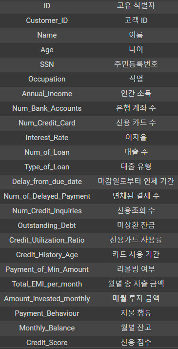
# 필요 없는 컬럼 삭제
credit_df.drop(['ID', 'Customer_ID','Name', 'SSN'], axis=1, inplace=True)

credit_df.info()
<class 'pandas.core.frame.DataFrame'>
RangeIndex: 12500 entries, 0 to 12499
Data columns (total 20 columns):
 #   Column                    Non-Null Count  Dtype
---  ------                    --------------  -----
 0   Age                       12500 non-null  object
 1   Occupation                12500 non-null  object
 2   Annual_Income             12500 non-null  object
 3   Num_Bank_Accounts         12500 non-null  int64
 4   Num_Credit_Card           12500 non-null  int64
 5   Interest_Rate             12500 non-null  int64
 6   Num_of_Loan               12500 non-null  object
 7   Type_of_Loan              11074 non-null  object
 8   Delay_from_due_date       12500 non-null  int64
 9   Num_of_Delayed_Payment    11657 non-null  object
 10  Num_Credit_Inquiries      12264 non-null  float64
 11  Outstanding_Debt          12500 non-null  object
 12  Credit_Utilization_Ratio  12500 non-null  float64
 13  Credit_History_Age        11387 non-null  object
 14  Payment_of_Min_Amount     12500 non-null  object
 15  Total_EMI_per_month       12500 non-null  float64
 16  Amount_invested_monthly   11935 non-null  object
 17  Payment_Behaviour         12500 non-null  object
 18  Monthly_Balance           12366 non-null  float64
 19  Credit_Score              12500 non-null  object
dtypes: float64(4), int64(4), object(12)
memory usage: 1.9+ MB
# 다중 클래스 분류
credit_df['Credit_Score'].value_counts()
Standard 6943
Poor 3582
Good 1975
Name: Credit_Score, dtype: int64
# object > int로 바꾸기
credit_df['Credit_Score'] = credit_df['Credit_Score'].replace({'Poor': 0, 'Standard': 1, 'Good': 2})credit_df.describe()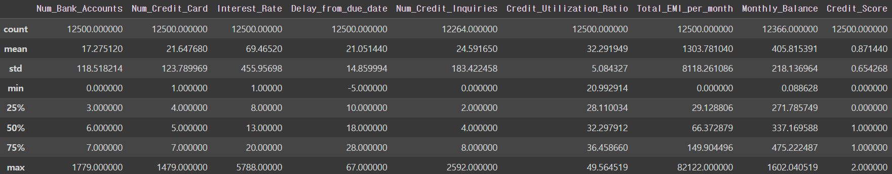
sns.barplot(x='Payment_of_Min_Amount', y='Credit_Score', data=credit_df)
plt.figure(figsize= (20, 5))
sns.barplot(x='Occupation', y='Credit_Score', data=credit_df)
# 컬럼 관련성 보기
plt.figure(figsize=(12,12))
sns.heatmap(credit_df.corr(),cmap='coolwarm', vmin= -1, vmax=1, annot=True)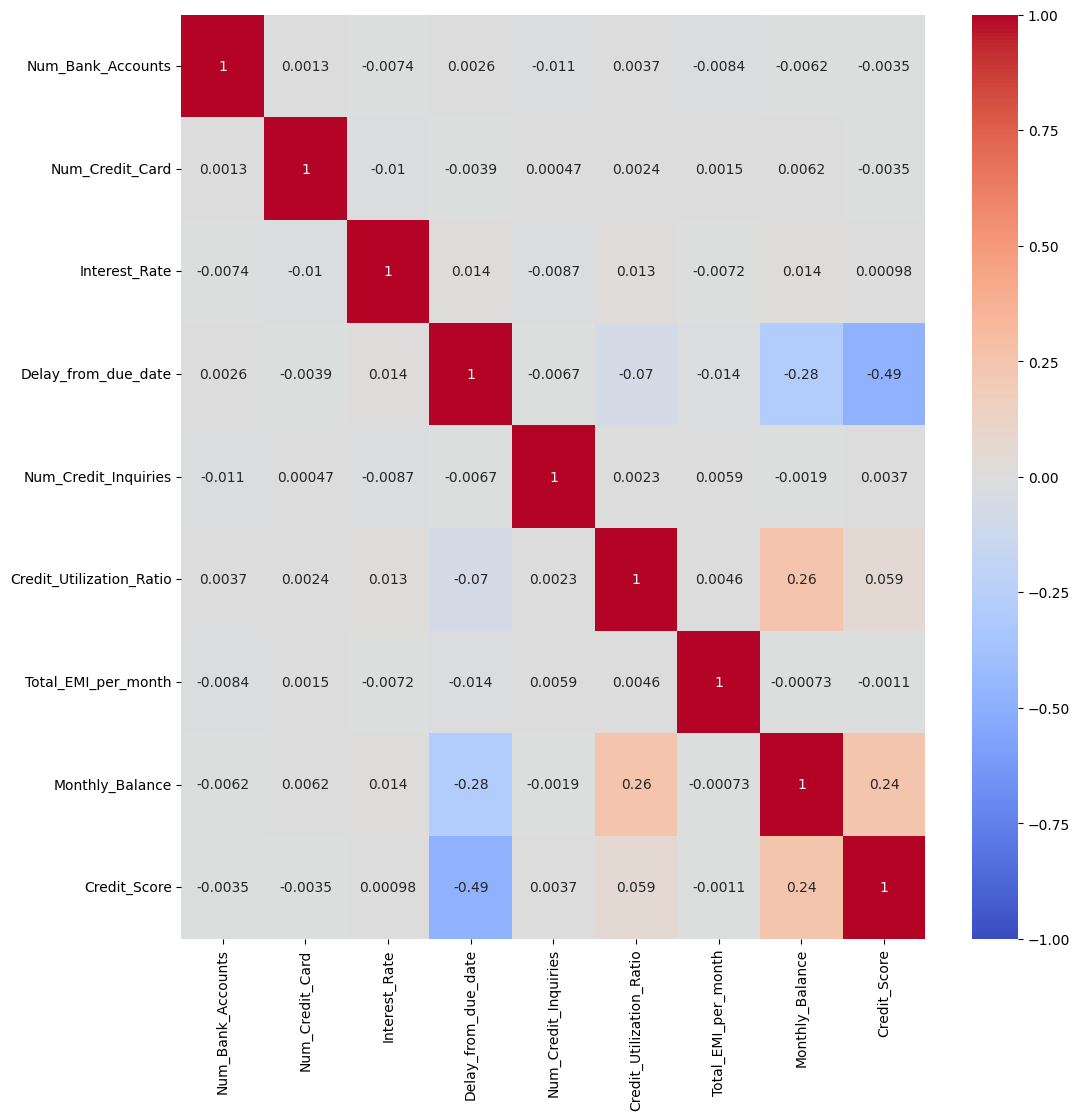
# object 타입 컬럼 보기
for i in credit_df.columns:
    if credit_df[i].dtype == 'O':
        print(i)
Age
Occupation
Annual_Income
Num_of_Loan
Type_of_Loan
Num_of_Delayed_Payment
Outstanding_Debt
Credit_History_Age
Payment_of_Min_Amount
Amount_invested_monthly
Payment_Behaviour
- 이상치 처리하기
# int 형식이지만 중간에 특수문자'_'가 들어가서 object타입인 컬럼들 고치기
for i in ['Age','Annual_Income', 'Num_of_Loan', 'Num_of_Delayed_Payment', 'Outstanding_Debt', 'Amount_invested_monthly']:
    credit_df[i] = pd.to_numeric(credit_df[i].str.replace('_',""))
credit_df.info()
<class 'pandas.core.frame.DataFrame'>
RangeIndex: 12500 entries, 0 to 12499
Data columns (total 20 columns):
# Column Non-Null Count Dtype
--- ------ -------------- -----
0 Age 12500 non-null int64
1 Occupation 12500 non-null object
2 Annual_Income 12500 non-null float64
3 Num_Bank_Accounts 12500 non-null int64
4 Num_Credit_Card 12500 non-null int64
5 Interest_Rate 12500 non-null int64
6 Num_of_Loan 12500 non-null int64
7 Type_of_Loan 11074 non-null object
8 Delay_from_due_date 12500 non-null int64
9 Num_of_Delayed_Payment 11657 non-null float64
10 Num_Credit_Inquiries 12264 non-null float64
11 Outstanding_Debt 12500 non-null float64
12 Credit_Utilization_Ratio 12500 non-null float64
13 Credit_History_Age 11387 non-null object
14 Payment_of_Min_Amount 12500 non-null object
15 Total_EMI_per_month 12500 non-null float64
16 Amount_invested_monthly 11935 non-null float64
17 Payment_Behaviour 12500 non-null object
18 Monthly_Balance 12366 non-null float64
19 Credit_Score 12500 non-null int64
dtypes: float64(8), int64(7), object(5)
memory usage: 1.9+ MB# Credit_History_Age의 데이터를 개월로 변경
예) 22 Years and 1 Months -> 22 * 12 + 1
credit_df['Credit_History_Age'] = credit_df['Credit_History_Age'].str.replace(' Months','')
credit_df['Credit_History_Age'] =
pd.to_numeric(credit_df['Credit_History_Age'].str.split(' Years and ',expand = True)[0])*12
+ pd.to_numeric(credit_df['Credit_History_Age'].str.split(' Years and ',expand = True)[1])
# 다른 방법
credit_df['New_Credit_History_Age'] = credit_df['Credit_History_Age'].apply(lambda x: int(x.split(' ')[0]) * 12 + int(x.split(' ')[-2]) if pd.notna(x) else 0)
credit_df['New_Credit_History_Age']credit_df.describe()
credit_df[credit_df['Age'] < 0]
// 115 rows × 20 columns

credit_df = credit_df[credit_df['Age'] >= 0]
credit_df.sort_values('Age').tail(20)
sns.boxplot(y=credit_df['Age'])
credit_df[credit_df['Age']>= 100].sort_values('Age')
// 260 rows × 20 columns
# 100살이 넘는 사람 데이터가 260개
# 110살 넘지 않는 데이터로만 다시 저장
credit_df = credit_df[credit_df['Age'] < 110]
✔️ 은행계좌가 10개 이상인 사람의 비율 확인
len(credit_df[credit_df['Num_Bank_Accounts'] > 10]) / len(credit_df)
// 0.013029853207982847
credit_df = credit_df[credit_df['Num_Bank_Accounts'] <= 10]len(credit_df[credit_df['Num_Credit_Card'] > 20]) / len(credit_df)
// 0.021975267379679145
credit_df = credit_df[credit_df['Num_Credit_Card'] <= 20]credit_df = credit_df[credit_df['Interest_Rate'] <= 40]
credit_df = credit_df[(credit_df['Num_of_Loan'] <= 10) & (credit_df['Num_of_Loan'] >= 0)]
credit_df = credit_df[credit_df['Delay_from_due_date'] >= 0]len(credit_df[credit_df['Num_of_Delayed_Payment'] > 30])
// 80
credit_df = credit_df[(credit_df['Num_of_Delayed_Payment'] <= 30) & (credit_df['Num_of_Delayed_Payment'] >= 0)]credit_df.info()
<class 'pandas.core.frame.DataFrame'>
Int64Index: 10004 entries, 0 to 12498
Data columns (total 20 columns):
# Column Non-Null Count Dtype
--- ------ -------------- -----
0 Age 10004 non-null int64
1 Occupation 10004 non-null object
2 Annual_Income 10004 non-null float64
3 Num_Bank_Accounts 10004 non-null int64
4 Num_Credit_Card 10004 non-null int64
5 Interest_Rate 10004 non-null int64
6 Num_of_Loan 10004 non-null int64
7 Type_of_Loan 8893 non-null object
8 Delay_from_due_date 10004 non-null int64
9 Num_of_Delayed_Payment 10004 non-null float64
10 Num_Credit_Inquiries 9816 non-null float64
11 Outstanding_Debt 10004 non-null float64
12 Credit_Utilization_Ratio 10004 non-null float64
13 Credit_History_Age 9106 non-null float64
14 Payment_of_Min_Amount 10004 non-null object
15 Total_EMI_per_month 10004 non-null float64
16 Amount_invested_monthly 9549 non-null float64
17 Payment_Behaviour 10004 non-null object
18 Monthly_Balance 9895 non-null float64
19 Credit_Score 10004 non-null int64
dtypes: float64(9), int64(7), object(4)
memory usage: 1.6+ MB- 결측치 확인
credit_df['Num_Credit_Inquiries'] = credit_df['Num_Credit_Inquiries'].fillna(0)credit_df.isna().mean()
Age 0.000000
Occupation 0.000000
Annual_Income 0.000000
Num_Bank_Accounts 0.000000
Num_Credit_Card 0.000000
Interest_Rate 0.000000
Num_of_Loan 0.000000
Type_of_Loan 0.111056
Delay_from_due_date 0.000000
Num_of_Delayed_Payment 0.000000
Num_Credit_Inquiries 0.000000
Outstanding_Debt 0.000000
Credit_Utilization_Ratio 0.000000
Credit_History_Age 0.089764
Payment_of_Min_Amount 0.000000
Total_EMI_per_month 0.000000
Amount_invested_monthly 0.045482
Payment_Behaviour 0.000000
Monthly_Balance 0.010896
Credit_Score 0.000000
dtype: float64sns.displot(credit_df['Credit_History_Age'])
sns.displot(credit_df['Amount_invested_monthly'])

sns.displot(credit_df['Monthly_Balance'])
# 한쪽으로 치우쳐진 데이터가 많기때문에 평균이 아닌 중앙값으로 결측치 대체
credit_df= credit_df.fillna(credit_df.median())
credit_df.isna().mean()
Age 0.000000
Occupation 0.000000
Annual_Income 0.000000
Num_Bank_Accounts 0.000000
Num_Credit_Card 0.000000
Interest_Rate 0.000000
Num_of_Loan 0.000000
Type_of_Loan 0.111056
Delay_from_due_date 0.000000
Num_of_Delayed_Payment 0.000000
Num_Credit_Inquiries 0.000000
Outstanding_Debt 0.000000
Credit_Utilization_Ratio 0.000000
Credit_History_Age 0.000000
Payment_of_Min_Amount 0.000000
Total_EMI_per_month 0.000000
Amount_invested_monthly 0.000000
Payment_Behaviour 0.000000
Monthly_Balance 0.000000
Credit_Score 0.000000
dtype: float64
# 문제.
# type_of_Loan의 모든 대출 상품을 변수에 저장
# 각 대출 상품에 대한 이름으로 컬럼을 만들고 대출 상품이 있는 경우 해당 컬럼에 1을 저장(원 핫 인코딩 방식)
credit_df['Type_of_Loan'] = credit_df['Type_of_Loan'].str.replace('and ', '')
credit_df['Type_of_Loan'] = credit_df['Type_of_Loan'].fillna('No Loan')
type_list = set(credit_df['Type_of_Loan'].str.split(', ').sum())
type_list
{'Auto Loan',
 'Credit-Builder Loan',
 'Debt Consolidation Loan',
 'Home Equity Loan',
 'Mortgage Loan',
 'No Loan',
 'Not Specified',
 'Payday Loan',
 'Personal Loan',
 'Student Loan'}
for i in type_list:
credit_df[i]= credit_df['Type_of_Loan'].apply(lambda x: 1 if i in x else 0)
credit_df.drop('Type_of_Loan', axis=1, inplace=True)
credit_df.info()

<class 'pandas.core.frame.DataFrame'>
Int64Index: 10004 entries, 0 to 12498
Data columns (total 29 columns):
 #   Column                    Non-Null Count  Dtype
---  ------                    --------------  -----
 0   Age                       10004 non-null  int64
 1   Occupation                10004 non-null  object
 2   Annual_Income             10004 non-null  float64
 3   Num_Bank_Accounts         10004 non-null  int64
 4   Num_Credit_Card           10004 non-null  int64
 5   Interest_Rate             10004 non-null  int64
 6   Num_of_Loan               10004 non-null  int64
 7   Delay_from_due_date       10004 non-null  int64
 8   Num_of_Delayed_Payment    10004 non-null  float64
 9   Num_Credit_Inquiries      10004 non-null  float64
 10  Outstanding_Debt          10004 non-null  float64
 11  Credit_Utilization_Ratio  10004 non-null  float64
 12  Credit_History_Age        10004 non-null  float64
 13  Payment_of_Min_Amount     10004 non-null  object
 14  Total_EMI_per_month       10004 non-null  float64
 15  Amount_invested_monthly   10004 non-null  float64
 16  Payment_Behaviour         10004 non-null  object
 17  Monthly_Balance           10004 non-null  float64
 18  Credit_Score              10004 non-null  int64
 19  No Loan                   10004 non-null  int64
 20  Auto Loan                 10004 non-null  int64
 21  Debt Consolidation Loan   10004 non-null  int64
 22  Mortgage Loan             10004 non-null  int64
 23  Not Specified             10004 non-null  int64
 24  Home Equity Loan          10004 non-null  int64
 25  Personal Loan             10004 non-null  int64
 26  Student Loan              10004 non-null  int64
 27  Credit-Builder Loan       10004 non-null  int64
 28  Payday Loan               10004 non-null  int64
dtypes: float64(9), int64(17), object(3)
memory usage: 2.3+ MB
credit_df['Occupation'].value_counts()
_______ 674
Lawyer 664
Mechanic 646
Scientist 640
Engineer 640
Architect 633
Teacher 624
Developer 621
Entrepreneur 620
Media_Manager 616
Accountant 611
Doctor 608
Musician 607
Journalist 606
Manager 602
Writer 592
Name: Occupation, dtype: int64# 어차피 모델은 카테고리로 인식하기때문에 꼭 바꿔줘야하는건 아니지만, 보기 편하게 변경 진행
credit_df['Occupation'] = credit_df['Occupation'].replace('_______', 'Unknown')
credit_df['Occupation'].value_counts()
Unknown          674
Lawyer           664
Mechanic         646
Scientist        640
Engineer         640
Architect        633
Teacher          624
Developer        621
Entrepreneur     620
Media_Manager    616
Accountant       611
Doctor           608
Musician         607
Journalist       606
Manager          602
Writer           592
Name: Occupation, dtype: int64
credit_df['Payment_Behaviour'].value_counts()
Low_spent_Small_value_payments 2506
High_spent_Medium_value_payments 1794
High_spent_Large_value_payments 1453
Low_spent_Medium_value_payments 1376
High_spent_Small_value_payments 1136
Low_spent_Large_value_payments 995
!@9#%8 744 # 알 수 없는 값이 있음
Name: Payment_Behaviour, dtype: int64credit_df['Payment_Behaviour'] = credit_df['Payment_Behaviour'].str.replace('!@9#%8','Unknown')
credit_df['Payment_Behaviour'].value_counts()
Low_spent_Small_value_payments 2506
High_spent_Medium_value_payments 1794
High_spent_Large_value_payments 1453
Low_spent_Medium_value_payments 1376
High_spent_Small_value_payments 1136
Low_spent_Large_value_payments 995
Unknown 744
Name: Payment_Behaviour, dtype: int64credit_df = pd.get_dummies(credit_df, columns = {'Payment_Behaviour','Occupation','Payment_of_Min_Amount'})2. lightGBM(LGBM)
Microsoft에서 개발한 LightGBM은 리프 중심 히스토그램 기반의 Gradient Boosting Framework로, 효율적이고 빠른 학습을 제공합니다. GBM은 모델 간의 앙상블을 통해 예측 정확도를 향상시키는 부스팅 알고리즘입니다. LightGBM은 이를 모델1을 통해 y를 예측하고, 모델2, 모델3에 차례로 데이터를 넣어 y를 예측하는 방식으로 구현합니다.
앙상블 모델
앙상블은 여러 개별 모델을 결합하여 하나의 강력한 모델을 형성하는 기술입니다. 이는 각 모델의 약점을 서로 보완하고 강점을 결합하여 높은 정확도와 안정성을 달성하는 데 도움이 됩니다. 1
junyealim.tistory.com
- LightGBM은 대용량 데이터셋에서 다른 Gradient Boosting 알고리즘보다 빠르게 학습됩니다. 특히 작은 데이터셋에서도 높은 성능을 보여줍니다.
- 메모리 사용량이 비교적 적어 대용량 데이터셋을 다룰 때에도 효율적으로 동작합니다.
- 과적합을 방지하기 위해 LightGBM은 조기 중단을 지원합니다. 이를 통해 모델의 학습을 일찍 멈출 수 있어, 불필요한 계산을 줄일 수 있습니다.
LightGBM은 작은 데이터셋에서 과적합 가능성이 높습니다. 일반적으로 10,000개 이상의 데이터셋을 사용하는 것이 권장됩니다.
from sklearn.model_selection import train_test_split
X_train, X_test, y_train, y_test = train_test_split(credit_df.drop('Credit_Score', axis=1),credit_df['Credit_Score'], test_size= 0.2, random_state=2023)
X_train.shape, y_train.shape // ((8003, 51), (8003,))
X_test.shape, y_test.shape // ((2001, 51), (2001,))
from lightgbm import LGBMClassifier
base_model = LGBMClassifier(random_state=2023)
base_model.fit(X_train,y_train)
pred = base_model.predict(X_test)from sklearn.metrics import accuracy_score, confusion_matrix, classification_report, roc_auc_scoreaccuracy_score(y_test, pred)
// 0.7251374312843578
confusion_matrix(y_test,pred)
//array([[409, 144, 25],
[154, 855, 108],
[ 4, 115, 187]])
print(classification_report(y_test, pred))
precision recall f1-score support
0 0.72 0.71 0.71 578
1 0.77 0.77 0.77 1117
2 0.58 0.61 0.60 306
accuracy 0.73 2001
macro avg 0.69 0.69 0.69 2001
weighted avg 0.73 0.73 0.73 2001
proba = base_model.predict_proba(X_test)
array([[1.85999520e-01, 5.12892812e-01, 3.01107668e-01],
[3.00755505e-02, 9.69418975e-01, 5.05474881e-04],
[1.77775175e-01, 4.70635184e-01, 3.51589641e-01],
...,
[6.05786945e-02, 6.17182265e-01, 3.22239040e-01],
[2.39508935e-01, 7.60120500e-01, 3.70565507e-04],
[2.00383699e-02, 9.79857031e-01, 1.04599097e-04]])
# 1.85999520e-01, 5.12892812e-01, 3.01107668e-01
# (0.18599952, 0.512892812, 0.301107668)roc_auc_score(y_test,proba, multi_class='ovr')
// 0.8932634160489487# 다중 클래스 분류여서 multi_class 항목을 선택해주어야한다! 대부분 OvR 전략 사용
- OvR(One-vs-Rest): 각 클래스마다 하나의 이진 분류기를 생성하고, 해당 클래스를 기준으로 그 클래스와 나머지 모든 클래스를 구분하는 이진 분류를 수행합니다. 가장 높은 확률을 가진 클래스를 선택합니다.
- OvO(One-vs-One): 클래스의 개수가 N이면 N(N-1)/2개의 이진 분류기를 만들어 각각 두 클래스를 구분합니다. 입력 데이터를 각 이진 분류기에 통과시켜 가장 많이 선택된 클래스를 최종 클래스로 선택합니다.
✔️리프 중심 히스토그램 기반 알고리즘
트리를 균형적으로 분할하는 것이 아니라, 최대한 불균형하게 분할하는 부스팅 프로그램의 성격
특성들의 분포를 히스토그램으로 나타내고, 해당 히스토그램을 이용하여 빠르게 후보 분할 기준을 선택
후보 분할 기준 중에서 최적의 분할 기준을 선택하기 위해, 데이터 포인트들을 히스토그램에 올바르게 배치하고, 이용하여 최적의 분할 기준을 선택함
앙상블 모델
앙상블은 여러 개별 모델을 결합하여 하나의 강력한 모델을 형성하는 기술입니다. 이는 각 모델의 약점을 서로 보완하고 강점을 결합하여 높은 정확도와 안정성을 달성하는 데 도움이 됩니다. 1
junyealim.tistory.com
3-1. 그래디언트 부스팅에 lightGBM 참고


