
1. 데이터 전처리
import numpy as np
import pandas as pd
import matplotlib.pyplot as plt
import seaborn as sns
bike_df = pd.read_csv('/content/drive/MyDrive/KDT/머신러닝과 딥러닝/data/bike.csv')
bike_df.info()
<class 'pandas.core.frame.DataFrame'>
RangeIndex: 33379 entries, 0 to 33378
Data columns (total 16 columns):
# Column Non-Null Count Dtype
--- ------ -------------- -----
0 datetime 33379 non-null object
1 count 33379 non-null int64
2 holiday 33379 non-null int64
3 workingday 33379 non-null int64
4 temp 33379 non-null float64
5 feels_like 33379 non-null float64
6 temp_min 33379 non-null float64
7 temp_max 33379 non-null float64
8 pressure 33379 non-null int64
9 humidity 33379 non-null int64
10 wind_speed 33379 non-null float64
11 wind_deg 33379 non-null int64
12 rain_1h 6771 non-null float64
13 snow_1h 326 non-null float64
14 clouds_all 33379 non-null int64
15 weather_main 33379 non-null object
dtypes: float64(7), int64(7), object(2)
memory usage: 4.1+ MB- datetime: 날짜
- count: 대여 개수
- holiday: 휴일
- workingday: 근무일
- temp: 기온
- feels_like: 체감온도
- temp_min: 최저온도
- temp_max: 최고온도
- pressure: 기압
- humidity: 습도
- wind_speed: 풍속
- wind_deg: 풍향
- rain_1h: 1시간당 내리는 비의 양
- snow_1h: 1시간당 내리는 눈의 양
- clouds_all: 구름의 양
- weather_main: 날씨
bike_df.describe()
sns.displot(bike_df['count'])
sns.boxplot(y=bike_df['count'])
✔️ 값들이 모두 연속되어 있기 때문에 이상치라고 판단하기 어렵다.
# 체감온도와 대여횟수 관계
sns.scatterplot(x='feels_like', y='count', data=bike_df, alpha=0.3)
sns.scatterplot(x='pressure', y='count', data=bike_df, alpha = 0.3)
sns.scatterplot(x='wind_speed', y='count', data=bike_df, alpha = 0.3)
sns.scatterplot(x='wind_deg', y='count', data=bike_df, alpha = 0.3)
- 결측값 확인
bike_df.isna().sum()

datetime            0
count               0
holiday             0
workingday          0
temp                0
feels_like          0
temp_min            0
temp_max            0
pressure            0
humidity            0
wind_speed          0
wind_deg            0
rain_1h         26608
snow_1h         33053
clouds_all          0
weather_main        0
dtype: int64
1시간 동안 온 비의 양과 눈의 양만 NaN값인 것은 비나 눈이 오지 않은 날을 뜻함을 알 수 있음
NaN => 0으로 채우기
bike_df = bike_df.fillna(0)

bike_df.isna().sum()
# NaN값 사라짐
datetime        0
count           0
holiday         0
workingday      0
temp            0
feels_like      0
temp_min        0
temp_max        0
pressure        0
humidity        0
wind_speed      0
wind_deg        0
rain_1h         0
snow_1h         0
clouds_all      0
weather_main    0
dtype: int64
bike_df.info()
# datetime, weather_main이 현재 object
<class 'pandas.core.frame.DataFrame'>
RangeIndex: 33379 entries, 0 to 33378
Data columns (total 16 columns):
# Column Non-Null Count Dtype
--- ------ -------------- -----
0 datetime 33379 non-null object
1 count 33379 non-null int64
2 holiday 33379 non-null int64
3 workingday 33379 non-null int64
4 temp 33379 non-null float64
5 feels_like 33379 non-null float64
6 temp_min 33379 non-null float64
7 temp_max 33379 non-null float64
8 pressure 33379 non-null int64
9 humidity 33379 non-null int64
10 wind_speed 33379 non-null float64
11 wind_deg 33379 non-null int64
12 rain_1h 33379 non-null float64
13 snow_1h 33379 non-null float64
14 clouds_all 33379 non-null int64
15 weather_main 33379 non-null object
dtypes: float64(7), int64(7), object(2)
memory usage: 4.1+ MBbike_df['datetime'] = pd.to_datetime(bike_df['datetime'])
bike_df.info()
<class 'pandas.core.frame.DataFrame'>
RangeIndex: 33379 entries, 0 to 33378
Data columns (total 16 columns):
# Column Non-Null Count Dtype
--- ------ -------------- -----
0 datetime 33379 non-null datetime64[ns]
1 count 33379 non-null int64
2 holiday 33379 non-null int64
3 workingday 33379 non-null int64
4 temp 33379 non-null float64
5 feels_like 33379 non-null float64
6 temp_min 33379 non-null float64
7 temp_max 33379 non-null float64
8 pressure 33379 non-null int64
9 humidity 33379 non-null int64
10 wind_speed 33379 non-null float64
11 wind_deg 33379 non-null int64
12 rain_1h 33379 non-null float64
13 snow_1h 33379 non-null float64
14 clouds_all 33379 non-null int64
15 weather_main 33379 non-null object
dtypes: datetime64[ns](1), float64(7), int64(7), object(1)
memory usage: 4.1+ MBbike_df['year'] = bike_df['datetime'].dt.year
bike_df['month'] = bike_df['datetime'].dt.month
bike_df['hour'] = bike_df['datetime'].dt.hour
bike_df['date'] = bike_df['datetime'].dt.date
plt.figure(figsize=(14,4))
sns.lineplot(x='date', y='count',data = bike_df)
plt.xticks(rotation=45)
plt.show()
- 선 그래프는 데이터 마지막과 시작부분을 선으로 이어버리기 때문에 2020년 1월~7월 사이에 잠시 데이터가 없음을 확인 할 수 있습니다.
# 2019년도 월 확인
bike_df[bike_df['year']==2019].groupby('month')['count'].mean()

month
1     193.368862
2     221.857718
3     326.564456
4     482.931694
5     438.027848
6     478.480053
7     472.745785
8     481.267366
9     500.862069
10    446.279070
11    307.295393
12    213.148886
Name: count, dtype: float64
bike_df[bike_df['year']==2020].groupby('month')['count'].mean()
month
1 260.445997
2 255.894320
3 217.135241
5 196.581064
6 290.900937
7 299.811688
8 331.528809
9 338.876478
10 293.640777
11 240.507324
12 138.993540
Name: count, dtype: float64- 2020년도 4월이 없음을 확인 할 수 있음
# covid로 컬럼 추가하기
# 2020-04-01 이전 : precovid
# 2020-04-01 이후 ~ 2021-05-01 이전: covid
# 2021-05-01 이후 : postcovid
# 함수 만들어서 적용하는 방법
bike_df['covid'] = 'precovid'

def covid(date):
    if str(date) < '2020-04-01':
        return 'precovid'
    elif str(date) < '2021-04-01':
        return 'covid'
    else:
        return 'postcovid'

bike_df['date'].apply(covid)
0         precovid
1         precovid
2         precovid
3         precovid
4         precovid
           ...
33374    postcovid
33375    postcovid
33376    postcovid
33377    postcovid
33378    postcovid
Name: date, Length: 33379, dtype: object
# lambda함수 이용하기
bike_df['covid'] = bike_df['date'].apply(lambda date: 'precovid' if str(date) < '2020-04-01' else 'covid' if str(date) < '2021-04-01' else 'postcovid')
- 날짜 계절로 변경하기
# 12월~2월 : winter
# 3월~5월: spring
# 6월~ 8월: summer
# 9월~11월: fall
bike_df['season'] = bike_df['month'].apply(lambda x: 'winter' if x == 12 else 'fall' if x >= 9 else 'summer' if x > 6 else 'spring' if x >= 3 else 'winter')

bike_df[['month', 'season']].value_counts().sort_index()
month  season
1      winter    3212
2      winter    3037
3      spring    3183
4      spring    2226
5      spring    3149
6      spring    3008
7      summer    3066
8      summer    3069
9      fall      2297
10     fall      2368
11     fall      2277
12     winter    2487
dtype: int64
- 시간 구간으로 변경하기
# 21 이후 ~ : night
# 19 이후 ~ : late evening
# 17 이후 ~ : early evening
# 16 이후 ~ : late afternoon
# 13 이후 ~ : early afternoon
# 11 이후 ~ : late morning
# 5 이후 ~ : early morning
bike_df['day_night'] = bike_df['hour'].apply(lambda x: 'night' if x >= 21
                                             else 'late evening' if x >= 19
                                             else 'early evening' if x >= 17
                                             else 'late afternoon' if x >= 16
                                             else 'early afternoon' if x >= 13
                                             else 'late morning' if x >= 11
                                             else 'early morning' if x >= 5
                                             else 'night')
bike_df.columns
// Index(['datetime', 'count', 'holiday', 'workingday', 'temp', 'feels_like',
'temp_min', 'temp_max', 'pressure', 'humidity', 'wind_speed',
'wind_deg', 'rain_1h', 'snow_1h', 'clouds_all', 'weather_main', 'year',
'month', 'hour', 'date', 'covid', 'season', 'day_night'],
dtype='object')
# 변경 완료된 컬럼들은 삭제
bike_df.drop(['datetime','month','date','hour'], axis=1, inplace=True)
bike_df.info()
<class 'pandas.core.frame.DataFrame'>
RangeIndex: 33379 entries, 0 to 33378
Data columns (total 19 columns):
# Column Non-Null Count Dtype
--- ------ -------------- -----
0 count 33379 non-null int64
1 holiday 33379 non-null int64
2 workingday 33379 non-null int64
3 temp 33379 non-null float64
4 feels_like 33379 non-null float64
5 temp_min 33379 non-null float64
6 temp_max 33379 non-null float64
7 pressure 33379 non-null int64
8 humidity 33379 non-null int64
9 wind_speed 33379 non-null float64
10 wind_deg 33379 non-null int64
11 rain_1h 33379 non-null float64
12 snow_1h 33379 non-null float64
13 clouds_all 33379 non-null int64
14 weather_main 33379 non-null object
15 year 33379 non-null int64
16 covid 33379 non-null object
17 season 33379 non-null object
18 day_night 33379 non-null object
dtypes: float64(7), int64(8), object(4)
memory usage: 4.8+ MB
- 문자열 컬럼들 유니크한 값 갯수 알아보기
for i in ['weather_main','covid','season','day_night']:
    print(i, bike_df[i].nunique())

weather_main 11
covid 3
season 4
day_night 7

bike_df['weather_main'].unique()
// array(['Clouds', 'Clear', 'Snow', 'Mist', 'Rain', 'Fog', 'Drizzle',
         'Haze', 'Thunderstorm', 'Smoke', 'Squall'], dtype=object)
weather_main의 값이 11개나 되지만 개인의 판단으로 합치기 어려운 값들이기 때문에 그대로 원 핫 인코딩 진행
# 원 핫 인코딩
bike_df = pd.get_dummies(bike_df, columns = ['weather_main','covid','season','day_night'])

# 컬럼 개수 40개
2. 의사 결정 나무
의사 결정 나무는 데이터를 분석하고 패턴을 파악하여 결정 규칙을 나무 구조로 나타낸 기계학습 알고리즘 중 하나입니다. 이 모델은 분류와 회귀 문제에 모두 사용되며, 간단하면서도 강력한 특징을 가지고 있습니다.
- 지니계수(지니 불순도, Gini Impurity)
의사 결정 나무에서 사용되는 지니계수는 분류 문제에서 특정 노드의 불순도를 나타냅니다. 노드가 포함하는 클래스들이 혼잡되어 있는 정도를 나타내며, 0에서 1까지의 값을 가집니다. 값이 0에 가까울수록 노드의 불순도가 없음을 의미하며, 이를 통해 모델이 얼마나 잘 분류되었는지를 판단할 수 있습니다. 또한 로그 연산이 없어 계산이 상대적으로 빠르다는 장점이 있습니다.
- 엔트로피
엔트로피는 어떤 집합이나 데이터의 불확실성, 혼잡도를 나타내는데 사용되는 또 다른 지표입니다. 노드의 불순도를 측정하며, 0에서 무한대까지의 값을 가집니다. 값이 0에 가까울수록 노드의 불순도가 없음을 의미합니다. 엔트로피는 로그 연산이 포함되어 있어 계산이 복잡하지만, 더 정확한 불순도 측정을 제공합니다.
- 오버피팅(과적합 (Overfitting) )
의사 결정 나무는 학습 데이터에서는 정확하지만 테스트 데이터에서는 성과가 나쁠 수 있는 오버피팅 현상이 자주 발생합니다. 이를 방지하기 위해 사용되는 방법 중 두 가지가 있습니다.
- 사전 가지치기: 나무가 다 자라기 전에 알고리즘을 멈추는 방법입니다. 특정 깊이나 노드 개수 등을 제한하여 오버피팅을 방지합니다.
- 사후 가지치기: 나무를 끝까지 돌린 후에 밑에서부터 가지를 쳐나가는 방법입니다. 불필요한 가지를 제거하여 모델을 최적화합니다.
from sklearn.model_selection import train_test_split

X_train, X_test, y_train, y_test = train_test_split(bike_df.drop('count', axis=1), bike_df['count'], test_size=0.2, random_state=2023)
의사 결정 나무 사용하기
from sklearn.tree import DecisionTreeRegressor
dtr = DecisionTreeRegressor(random_state=2023)
# random_state=2023와 같이 모델에 들어가는 파라미터는 하이퍼파라미터라고 칭한다.
dtr.fit(X_train, y_train)
pred1 = dtr.predict(X_test)

sns.scatterplot(x = y_test, y = pred1)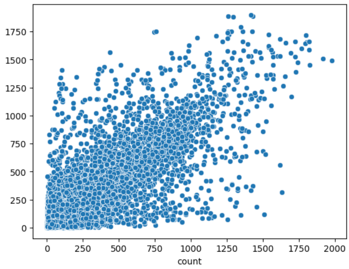
- 대각선 형태: 대각선 형태로 점들이 분포되는 것은 모델이 예측을 정확하게 했을 때입니다. 이는 정확한 예측값과 정답이 일치하는 경우를 나타냅니다.
- 가운데를 중심으로 밀집된 모습: 대다수의 점이 가운데를 중심으로 모여있을수록 모델이 전체적으로 일관된 예측을 수행했다는 것을 나타냅니다.
- 이탈된 이상치 없음: 이상치가 없거나 매우 적은 경우, 모델이 극단적인 값을 예측하는 경향이 낮아 좋은 성능을 나타낼 가능성이 높습니다.
위의 표를 통해서 대체적으로 예측이 잘 되었다는 점을 알 수 있습니다.
- RMSE 평가 지표 적용
from sklearn.metrics import mean_squared_error

mean_squared_error(y_test, pred1, squared=False)
// 222.11143591461095
3. 선형 회귀 VS 의사 결정 나무
from sklearn.linear_model import LinearRegression

lr = LinearRegression()
lr.fit(X_train, y_train)
pred2 =lr.predict(X_test)

sns.scatterplot(x = y_test, y=pred2)
- 평가 지표 적용
mean_squared_error(y_test, pred2, squared=False)
// 224.4795736198624
# 의사 결정 나무 : 222.11143591461095
# 선형 회귀 : 224.4795736198624
222.11143591461095 - 224.4795736198624
// -2.3681377052514563의사 결정 나무의 값이 더 작기 때문에 의사 결정 나무의 예측이 더 정확하다고 판단.
4. 하이퍼 파라미터 적용
dtr = DecisionTreeRegressor(random_state=2023, max_depth = 50, min_samples_leaf = 30)# min_samples_leaf : 의사 결정 나무 모델에서 잎 노드(leaf node)가 가져야 하는 최소 샘플 데이터 포인트 수를 지정하는 매개변수. 30의 값을 주면 만약 잎 노드에 속한 데이터의 수가 30보다 작으면, 추가적인 분기가 일어나지 않고 해당 노드에서 멈추게 됩니다. 값을 크게 설정할수록 각 잎 노드가 더 많은 데이터 포인트를 가져야 하므로, 트리의 깊이가 감소합니다. 이를 통해 모델이 훈련 데이터에 과적합되는 것을 방지하고, 더 간결하고 일반화된 모델을 얻을 수 있습니다.
dtr.fit(X_train, y_train)

pred3 = dtr.predict(X_test)
# 평가지표 적용
mean_squared_error(y_test, pred3, squared = False)
// 186.17062846092128
# 의사 결정 나무 : 222.11143591461095
# 의사 결정 나무(하이퍼 파라미터 튜닝) : 186.17062846092128
186.17062846092128 - 222.11143591461095
// -35.94080745368967하이퍼 파라미터 튜닝 후 더 정확한 예측을 함
plt.figure(figsize=(24,12))
plot_tree(dtr, max_depth= 5, fontsize=12)
plt.show()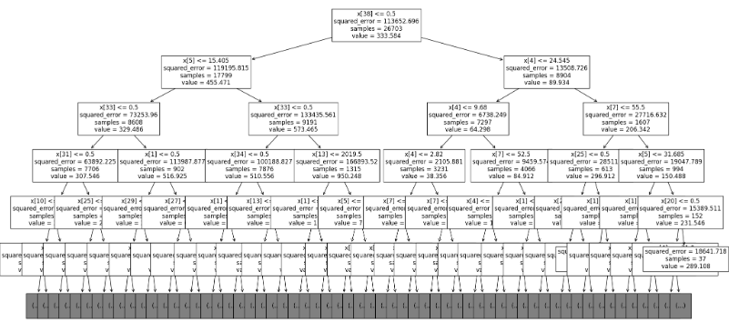
plt.figure(figsize=(24,12))
plot_tree(dtr, max_depth= 5, fontsize=12, feature_names = X_train.columns)
# 컬럼 이름 표시하기
plt.show()
'AI' 카테고리의 다른 글
| 서포트 벡터 머신 (0) | 2023.12.28 |
|---|---|
| 로지스틱 회귀 (0) | 2023.12.27 |
| 선형 회귀(랜트비 예측) (1) | 2023.12.26 |
| 타이타닉 데이터셋 (0) | 2023.12.26 |
| 사이킷런/아이리스 데이터셋 예제 (0) | 2023.12.24 |


