1. 데이터 전처리
import numpy as np
import pandas as pd
import seaborn as sns

rent_df = pd.read_csv('/content/drive/MyDrive/KDT/머신러닝과 딥러닝/data/rent.csv')
rent_df.info()

<class 'pandas.core.frame.DataFrame'>
RangeIndex: 4746 entries, 0 to 4745
Data columns (total 12 columns):
 #   Column             Non-Null Count  Dtype
---  ------             --------------  -----
 0   Posted On          4746 non-null   object
 1   BHK                4743 non-null   float64
 2   Rent               4746 non-null   int64
 3   Size               4741 non-null   float64
 4   Floor              4746 non-null   object
 5   Area Type          4746 non-null   object
 6   Area Locality      4746 non-null   object
 7   City               4746 non-null   object
 8   Furnishing Status  4746 non-null   object
 9   Tenant Preferred   4746 non-null   object
 10  Bathroom           4746 non-null   int64
 11  Point of Contact   4746 non-null   object
dtypes: float64(2), int64(2), object(8)
memory usage: 445.1+ KB- Posted On : 매물 등록 날짜
- BHK : 베드, 홀, 키친의 개수
- Rent : 렌트비
- Size : 집 크기
- Floor : 총 층수 중 몇 층
- Area Type : 공용공간을 포함하는지, 집의 면적만 포함하는지
- Area Locality : 지역
- City : 도시
- Furnishing Status : 풀옵션 여부
- Tenant Preferred : 선호하는 가족형태
- Bathroom : 화장실 개수
- Point of Contact : 연락할 곳
# .describe() 데이터프레임의 주요 통계적 특징을 요약하여 제공하는 함수
rent_df.describe()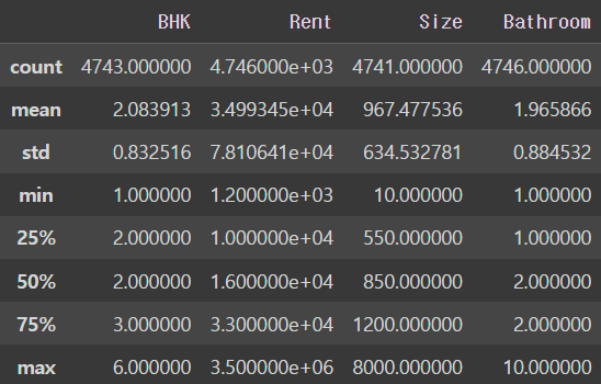
# round함수 통해 소숫점 2번째 자리까지만 표출
round(rent_df.describe(), 2)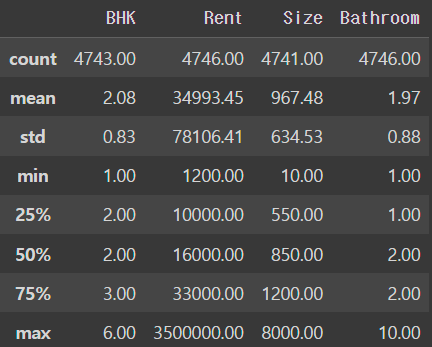
sns.displot(rent_df['BHK'])
sns.displot(rent_df['Rent'])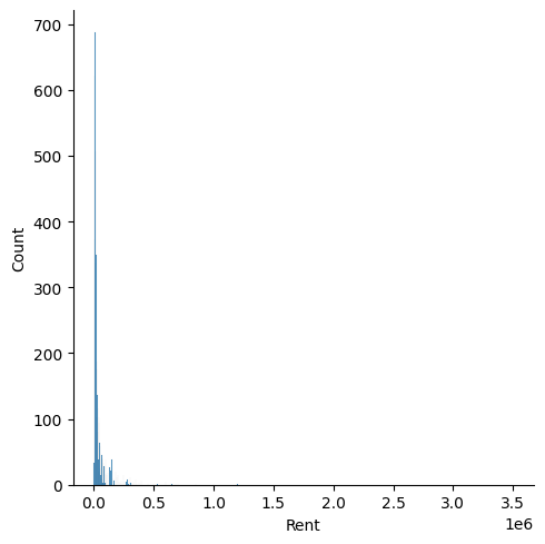
⭐ 렌트비처럼 공통값이 별로 없는 컬럼은 막대 그래프로 보는것은 좋지 않다.
rent_df['Rent'].sort_values()

4076       1200
285        1500
471        1800
2475       2000
146        2200
         ...
1459     700000
1329     850000
827     1000000
1001    1200000
1837    3500000
Name: Rent, Length: 4746, dtype: int64
- 이상치 확인하기
sns.boxplot(y=rent_df['Rent'])
sns.boxplot(y=rent_df['BHK'])
값의 차이가 크지 않아서(1씩밖에 차이나지 않음) 범위를 크게 벗어난 것이 아니기 때문에 이상치로 보기 어려움.
- 결측값 확인
rent_df.isna().sum()

Posted On            0
BHK                  3
Rent                 0
Size                 5
Floor                0
Area Type            0
Area Locality        0
City                 0
Furnishing Status    0
Tenant Preferred     0
Bathroom             0
Point of Contact     0
dtype: int64

rent_df.isna().mean()

Posted On            0.000000
BHK                  0.000632
Rent                 0.000000
Size                 0.001054
Floor                0.000000
Area Type            0.000000
Area Locality        0.000000
City                 0.000000
Furnishing Status    0.000000
Tenant Preferred     0.000000
Bathroom             0.000000
Point of Contact     0.000000
dtype: float64
- [BHK] 열의 결측값이 많지 않기에 NaN이 있는 행은 삭제하는 경우
# inplace = True 명시하지 않았기 때문에 원본 데이터가 변형되지는 않음
rent_df.dropna(subset=['BHK'])
- [size] 열의 결측값은 중앙값으로 대체.
# rent_df에서 Size가 NaN인 데이터의 index를 저장
na_index= rent_df[rent_df['Size'].isna()].index

na_index
// Int64Index([425, 430, 4703, 4731, 4732], dtype='int64')

rent_df.fillna(rent_df.median()).loc[na_index]
- [BHK] 열의 결측값도 중앙값으로 대체해보기.
na_index= rent_df[rent_df['BHK'].isna()].index

na_index // Int64Index([3, 53, 89], dtype='int64')

rent_df['BHK'].fillna(rent_df['BHK'].median()).loc[na_index]
3     2.0
53    2.0
89    2.0
Name: BHK, dtype: float64
# 모든 결측값 중앙값으로 대체 시
rent_df = rent_df.fillna(rent_df.median())
결측값 처리 완료
rent_df.isna().mean()

Posted On            0.0
BHK                  0.0
Rent                 0.0
Size                 0.0
Floor                0.0
Area Type            0.0
Area Locality        0.0
City                 0.0
Furnishing Status    0.0
Tenant Preferred     0.0
Bathroom             0.0
Point of Contact     0.0
dtype: float64

rent_df.info()

<class 'pandas.core.frame.DataFrame'>
RangeIndex: 4746 entries, 0 to 4745
Data columns (total 12 columns):
 #   Column             Non-Null Count  Dtype
---  ------             --------------  -----
 0   Posted On          4746 non-null   object
 1   BHK                4746 non-null   float64
 2   Rent               4746 non-null   int64
 3   Size               4746 non-null   float64
 4   Floor              4746 non-null   object
 5   Area Type          4746 non-null   object
 6   Area Locality      4746 non-null   object
 7   City               4746 non-null   object
 8   Furnishing Status  4746 non-null   object
 9   Tenant Preferred   4746 non-null   object
 10  Bathroom           4746 non-null   int64
 11  Point of Contact   4746 non-null   object
dtypes: float64(2), int64(2), object(8)
memory usage: 445.1+ KB
rent_df['Area Type'].value_counts()
Super Area 2446
Carpet Area 2298
Built Area 2
Name: Area Type, dtype: int64✔️ nunique() : 데이터프레임의 열에서 고유한(unique)한 값의 개수를 반환하는 함수
rent_df['Area Type'].unique()
// array(['Super Area', 'Carpet Area', 'Built Area'], dtype=object)

rent_df['Area Type'].nunique()
// 3
# object 타입의 컬럼
col = ['Floor', 'Area Type', 'Area Locality',
'Furnishing Status','Tenant Preferred', 'City', 'Point of Contact']
rent_df[['Floor', 'Area Type', 'Area Locality', 'Furnishing Status',
'Tenant Preferred','Point of Contact']].nunique()
Floor 480
Area Type 3
Area Locality 2235
Furnishing Status 3
Tenant Preferred 3
City 6
Point of Contact 3
dtype: int64# 렌트비와 관계가 적거나 원 핫 인코딩이 어려운 열들 삭제
rent_df.drop(['Floor', 'Area Locality', 'Tenant Preferred', 'Point of Contact',
'Posted On'], axis=1, inplace=True)
rent_df.info()
<class 'pandas.core.frame.DataFrame'>
RangeIndex: 4746 entries, 0 to 4745
Data columns (total 7 columns):
# Column Non-Null Count Dtype
--- ------ -------------- -----
0 BHK 4746 non-null float64
1 Rent 4746 non-null int64
2 Size 4746 non-null float64
3 Area Type 4746 non-null object
4 City 4746 non-null object
5 Furnishing Status 4746 non-null object
6 Bathroom 4746 non-null int64
dtypes: float64(2), int64(2), object(3)
memory usage: 259.7+ KB# 원 핫 인코딩
rent_df = pd.get_dummies(rent_df, columns = ['Area Type','City','Furnishing Status'])
rent_df.head()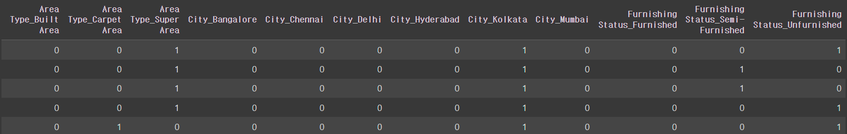
X = rent_df.drop('Rent', axis=1) # 독립변수
y = rent_df['Rent'] # 종속변수
from sklearn.model_selection import train_test_split
X_train, X_test,y_train, y_test= train_test_split(X, y, test_size = 0.2, random_state = 10)
X_train.shape, y_train.shape
// ((3796, 15), (3796,))
X_test.shape, y_test.shape
// ((950, 15), (950,))2. 선형 회귀(Linear Regression)
데이터를 통해 가장 잘 설명할 수 있는 직선으로 데이터를 분석하는 방법
- 단순 선형 회귀분석(단일 독립변수를 이용)
- 다중 선형 회귀분석(다중 독립변수를 이용)
from sklearn.linear_model import LinearRegression

lr = LinearRegression()
lr.fit(X_train, y_train)
pred = lr.predict(X_test)3. 평가지표
1. MSE (Mean Squared Error)
MSE는 실제 값과 예측 값 간의 제곱 오차를 모두 더한 후, 평균을 구한 값입니다.

MSE는 오차를 제곱하기 때문에 예측 값이 실제 값과 멀어질수록 더 큰 가중치를 가지게 됩니다.
p = np.array([3,4,5]) # 예측값
act = np.array([1,2,3]) # 실제값

def my_mse(pred, actual):
    return((pred-actual) **2).mean()

my_mse(p, act)
// 4.0
2. MAE (Mean Absolute Error)
MAE는 실제 값과 예측 값 간의 '절대값' 오차를 모두 더한 후, 평균을 구한 값입니다.

MAE는 예측 값과 실제 값 간의 차이를 제곱하지 않기 때문에 이상치(outlier)에 덜 민감합니다. (하지만 잘 사용하지 않음)
def my_mae(pred, actual):
    return np.abs(pred - actual).mean()

my_mae(p,act)
// 2.0
3. RMSE (Root Mean Squared Error)
RMSE는 MSE의 제곱근으로, 예측 오차의 제곱에 루트를 씌운 값입니다.


RMSE는 오차의 크기를 측정하며, 값이 작을수록 모델의 예측이 정확하다고 판단됩니다.
def my_rmse(pred, actual):
    return np.sqrt(my_mse(pred,actual))

my_rmse(p, act)
// 2.0
from sklearn.metrics import mean_absolute_error, mean_squared_error
mean_absolute_error(p,act) // 2.0
mean_squared_error(p, act) // 4.0
# RMSE
mean_squared_error(p, act , squared=False) // 2.04. 평가지표 적용하기
mean_squared_error(y_test, pred)
// 1717185779.0021067
mean_absolute_error(y_test, pred)
// 22779.17722543894
mean_squared_error(y_test, pred, squared=False)
// 41438.9403701652
- 이상치 삭제해보기
X_train.drop(1837, inplace=True)
y_train.drop(1837, inplace=True)
lr.fit(X_train, y_train)
pred = lr.predict(X_test)

mean_squared_error(y_test, pred, squared=False)
// 41377.57030234839
# 1837 삭제 전: 41438.9403701652
# 1837 삭제 후: 41377.57030234839
41438.9403701652 - 41377.57030234839
// 61.37006781680975오차가 줄어들었음
'AI' 카테고리의 다른 글
| 로지스틱 회귀 (0) | 2023.12.27 |
|---|---|
| 의사 결정 나무(자전거 대여 예제) (0) | 2023.12.26 |
| 타이타닉 데이터셋 (0) | 2023.12.26 |
| 사이킷런/아이리스 데이터셋 예제 (0) | 2023.12.24 |
| 머신러닝과 딥러닝 (0) | 2023.12.14 |


