
1. 단계별로 예시 보기
import torch
import torch.nn as nn
import torch.optim as optim
# 배치크기 / 채널(1 : 그레이스케일, 3: 컬러) / 높이 / 너비
inputs = torch.Tensor(1, 1, 28, 28)
print(inputs.shape) // torch.Size([1, 1, 28, 28])# 첫번째 Conv2D
# kernel_size=3 : 필터 사이즈. 3*3. 클수록 출력값이 작아짐
# padding='same' : 출력 크기 동일하게 유지
conv1 = nn.Conv2d(in_channels=1, out_channels=32, kernel_size=3, padding='same')
out = conv1(inputs)
print(out.shape) // torch.Size([1, 32, 28, 28])# 첫번째 MaxPool2D
pool = nn.MaxPool2d(kernel_size=2)
out = pool(out)
print(out.shape) // torch.Size([1, 32, 14, 14])# 이미지 사이즈가 kernel_size로 나눈만큼 줄어듬
# kernel_size는 높이,너비 나눠지게끔 맞춰야함
# 두번째 Conv2D
conv2 = nn.Conv2d(in_channels=32, out_channels=64, kernel_size=3, padding='same')
out = conv2(out)
print(out.shape) // torch.Size([1, 64, 14, 14])
# 두번째 MaxPool2D
pool = nn.MaxPool2d(kernel_size=2)
out = pool(out)
print(out.shape) // torch.Size([1, 64, 7, 7])flatten = nn.Flatten()
out = flatten(out)
print(out.shape) // torch.Size([1, 3136]) # 64*7*7 = 3136fc = nn.Linear(3136, 10)
out = fc(out)
print(out.shape) // torch.Size([1, 10])2. CNN으로 MNIST 분류하기
import torchvision.datasets as datasets
import torchvision.transforms as transforms
import matplotlib.pyplot as plt
from torch.utils.data import DataLoader
device = 'cuda' if torch.cuda.is_available() else 'cpu'
print(device) // cuda# torchvision.datasets에서 데이터 받아오는 법!
train_data = datasets.MNIST(
root = 'data',
train = True, # False로 주면 test데이터가 받아짐
transform= transforms.ToTensor(), # Tensor 형식으로 받아옴
download = True
)
test_data = datasets.MNIST(
root = 'data',
train = False, # test데이터가 받아짐
transform= transforms.ToTensor(),
download = True
)print(train_data)
// Dataset MNIST
Number of datapoints: 60000
Root location: data
Split: Train
StandardTransform
Transform: ToTensor()
print(test_data)
// Dataset MNIST
Number of datapoints: 10000
Root location: data
Split: Test
StandardTransform
Transform: ToTensor()# 데이터로더 만들기
# batch_size =64, shuffle = True
# 8*8 형태로 이미지를 출력
loader = DataLoader(
dataset = train_data,
batch_size = 64,
shuffle=True
)
imgs, labels = next(iter(loader))
print(imgs.shape)
fig, axes = plt.subplots(8, 8, figsize= (16, 16))
for ax, img, label in zip(axes.flatten(), imgs, labels):
ax.imshow(img.reshape((28,28)),cmap='gray')
ax.set_title(label.item())
ax.axis('off')
model = nn.Sequential(
    nn.Conv2d(1, 32, kernel_size=3, padding='same'),
    nn.ReLU(),
    nn.MaxPool2d(kernel_size=2),

    nn.Conv2d(32, 64, kernel_size=3, padding='same'),
    nn.ReLU(),
    nn.MaxPool2d(kernel_size=2),

    nn.Flatten(),
    nn.Linear(7*7*64, 10)
).to(device)
print(model)
Sequential(
(0): Conv2d(1, 32, kernel_size=(3, 3), stride=(1, 1), padding=same)
(1): ReLU()
(2): MaxPool2d(kernel_size=2, stride=2, padding=0, dilation=1, ceil_mode=False) # ceil_mode=True는 올림모드
(3): Conv2d(32, 64, kernel_size=(3, 3), stride=(1, 1), padding=same)
(4): ReLU()
(5): MaxPool2d(kernel_size=2, stride=2, padding=0, dilation=1, ceil_mode=False)
(6): Flatten(start_dim=1, end_dim=-1)
(7): Linear(in_features=3136, out_features=10, bias=True)
)
# 학습
# optimizer: Adam
# Epoch 10/10 Loss: 0.010452 Accuracy: 99.64%

optimizer = optim.Adam(model.parameters(), lr= 0.001)
epochs = 10

for epoch in range(epochs +1):
    sum_losses = 0
    sum_accs = 0

    # 64개씩 들어감. (데이터 갯수//64)번 반복
    for x_batch, y_batch in loader:
        # 모델이 GPU에 있기 때문에 데이터도 GPU로 보내줘야한다.
        x_batch, y_batch = x_batch.to(device), y_batch.to(device)
        y_pred = model(x_batch)
        loss = nn.CrossEntropyLoss()(y_pred, y_batch)

        optimizer.zero_grad()
        loss.backward()
        optimizer.step()

        sum_losses = sum_losses + loss

        y_prob = nn.Softmax(1)(y_pred)
        y_pred_index = torch.argmax(y_prob, axis=1)
        acc = (y_batch == y_pred_index).float().sum() / len(y_batch) * 100
        sum_accs = sum_accs + acc

    # epoch 한번 끝날때마다 업데이트 된 loss와 accuracy 평균 보기
    avg_loss = sum_losses / len(loader)
    avg_acc = sum_accs / len(loader)
    print(f'Epoch {epoch: 4d}/{epochs} Loss: {avg_loss: .6f} Accuracy: {avg_acc:.2f}%')
Epoch 0/10 Loss: 0.177507 Accuracy: 94.67%
Epoch 1/10 Loss: 0.055723 Accuracy: 98.33%
Epoch 2/10 Loss: 0.039588 Accuracy: 98.78%
Epoch 3/10 Loss: 0.032302 Accuracy: 98.99%
Epoch 4/10 Loss: 0.025851 Accuracy: 99.21%
Epoch 5/10 Loss: 0.021630 Accuracy: 99.32%
Epoch 6/10 Loss: 0.017488 Accuracy: 99.46%
Epoch 7/10 Loss: 0.014252 Accuracy: 99.55%
Epoch 8/10 Loss: 0.011443 Accuracy: 99.64%
Epoch 9/10 Loss: 0.009461 Accuracy: 99.68%
Epoch 10/10 Loss: 0.009722 Accuracy: 99.69%
# test_loader를 만들어 데이터를 출력
# batch_size = 64, shuffle = True
# 8*8 형태로 이미지를 출력
test_loader = DataLoader(
    dataset = test_data,
    batch_size = 64,
    shuffle=True
)

imgs, labels = next(iter(test_loader))

fig, axes = plt.subplots(8, 8, figsize= (16, 16))

for ax, img, label in zip(axes.flatten(), imgs, labels):
    ax.imshow(img.reshape((28,28)),cmap='gray')
    ax.set_title(label.item())
    ax.axis('off')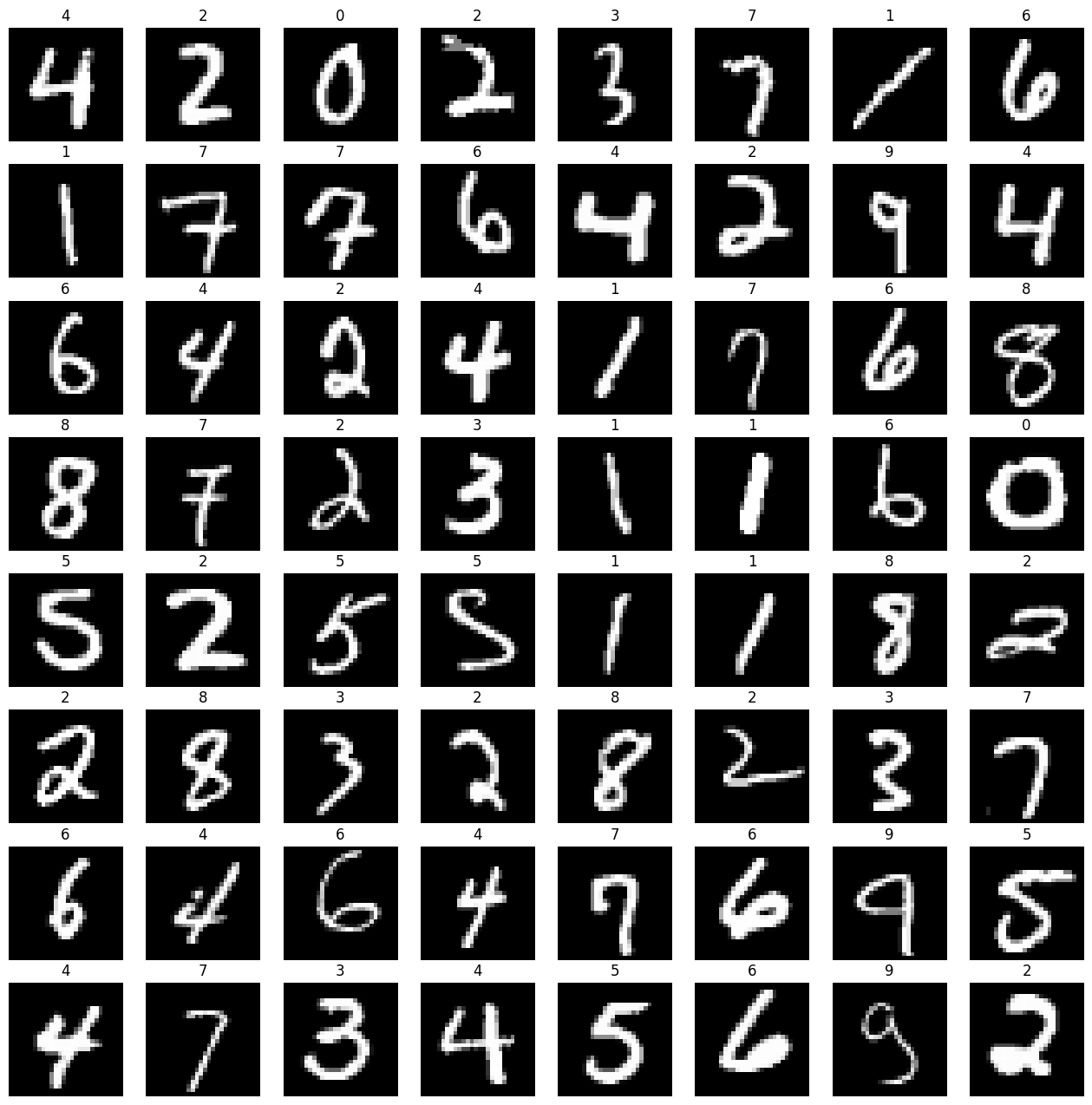
model.eval() # 모델을 테스트 모드로 전환
accs = 0
for imgs, labels in test_loader:
    imgs, labels = imgs.to(device), labels.to(device)
    y_pred = model(imgs)
    y_prob = nn.Softmax(1)(y_pred)
    y_pred_index = torch.argmax(y_prob, axis=1)
    accuracy = (labels == y_pred_index).float().sum() / len(imgs) * 100
    accs = accs + accuracy
avg_acc = accs / len(test_loader)
print(f'테스트 정확도는 {avg_acc: .2f}% 입니다!')
// 테스트 정확도는 99.01% 입니다!- 훈련 모드 (Training Mode): model.train()을 호출하여 모델을 훈련 모드로 전환합니다. 이때 드롭아웃이나 배치 정규화와 같은 학습 관련 동작들이 활성화됩니다.
- 평가 모드 (Evaluation Mode): model.eval()을 호출하여 모델을 평가 모드로 전환합니다. 이때 드롭아웃이나 배치 정규화와 같은 동작들이 비활성화되어 테스트나 검증 시 일관된 결과를 얻을 수 있습니다. 배치 정규화는 훈련 데이터의 통계를 사용하여 정규화를 수행하는데, 이를 평가할 때에는 테스트 데이터의 통계를 사용하여 일관성을 유지합니다.
'AI' 카테고리의 다른 글
| 포켓몬 분류 해보기 (1) | 2024.01.14 |
|---|---|
| 전이 학습 (0) | 2024.01.12 |
| CNN 기초 (0) | 2024.01.10 |
| 비선형 활성화 함수 (0) | 2024.01.10 |
| 딥러닝 (0) | 2024.01.09 |


